Munich-chain-ladder Model
MunichChainLadder.RdThe Munich-chain-ladder model forecasts ultimate claims based on a cumulative
paid and incurred claims triangle.
The model assumes that the Mack-chain-ladder model is applicable
to the paid and incurred claims triangle, see MackChainLadder.
Usage
MunichChainLadder(Paid, Incurred,
                  est.sigmaP = "log-linear", est.sigmaI = "log-linear",
                  tailP=FALSE, tailI=FALSE, weights=1)
Arguments
- Paid
cumulative paid claims triangle. Assume columns are the development period, use transpose otherwise. A (mxn)-matrix \(P_{ik}\) which is filled for \(k \leq n+1-i; i=1,\ldots,m; m\geq n\)
- Incurred
cumulative incurred claims triangle. Assume columns are the development period, use transpose otherwise. A (mxn)-matrix \(I_{ik}\) which is filled for \(k \leq n+1-i; i=1,\ldots,m, m\geq n \)
- est.sigmaP
defines how \(sigma_{n-1}\) for the Paid triangle is estimated, see
est.sigmainMackChainLadderfor more details, asest.sigmaPgets passed on toMackChainLadder- est.sigmaI
defines how \(sigma_{n-1}\) for the Incurred triangle is estimated, see
est.sigmainMackChainLadderfor more details, asest.sigmaIis passed on toMackChainLadder- tailP
defines how the tail of the
Paidtriangle is estimated and is passed on toMackChainLadder, seetailjust there.- tailI
defines how the tail of the
Incurredtriangle is estimated and is passed on toMackChainLadder, seetailjust there.- weights
weights. Default: 1, which sets the weights for all triangle entries to 1. Otherwise specify weights as a matrix of the same dimension as Triangle with all weight entries in [0; 1]. Hence, any entry set to 0 or NA eliminates that age-to-age factor from inclusion in the model. See also 'Details' in MackChainladder function. The weight matrix is the same for Paid and Incurred.
Value
MunichChainLadder returns a list with the following elements
- call
matched call
- Paid
input paid triangle
- Incurred
input incurred triangle
- MCLPaid
Munich-chain-ladder forecasted full triangle on paid data
- MCLIncurred
Munich-chain-ladder forecasted full triangle on incurred data
- MackPaid
Mack-chain-ladder output of the paid triangle
- MackIncurred
Mack-chain-ladder output of the incurred triangle
- PaidResiduals
paid residuals
- IncurredResiduals
incurred residuals
- QResiduals
paid/incurred residuals
- QinverseResiduals
incurred/paid residuals
- lambdaP
dependency coefficient between paid chain-ladder age-to-age factors and incurred/paid age-to-age factors
- lambdaI
dependency coefficient between incurred chain-ladder ratios and paid/incurred ratios
- qinverse.f
chain-ladder-link age-to-age factors of the incurred/paid triangle
- rhoP.sigma
estimated conditional deviation around the paid/incurred age-to-age factors
- q.f
chain-ladder age-to-age factors of the paid/incurred triangle
- rhoI.sigma
estimated conditional deviation around the incurred/paid age-to-age factors
Author
Markus Gesmann markus.gesmann@gmail.com
Examples
MCLpaid
#> dev
#> origin 1 2 3 4 5 6 7
#> 1 576 1804 1970 2024 2074 2102 2131
#> 2 866 1948 2162 2232 2284 2348 NA
#> 3 1412 3758 4252 4416 4494 NA NA
#> 4 2286 5292 5724 5850 NA NA NA
#> 5 1868 3778 4648 NA NA NA NA
#> 6 1442 4010 NA NA NA NA NA
#> 7 2044 NA NA NA NA NA NA
MCLincurred
#> dev
#> origin 1 2 3 4 5 6 7
#> 1 978 2104 2134 2144 2174 2182 2174
#> 2 1844 2552 2466 2480 2508 2454 NA
#> 3 2904 4354 4698 4600 4644 NA NA
#> 4 3502 5958 6070 6142 NA NA NA
#> 5 2812 4882 4852 NA NA NA NA
#> 6 2642 4406 NA NA NA NA NA
#> 7 5022 NA NA NA NA NA NA
op <- par(mfrow=c(1,2))
plot(MCLpaid)
plot(MCLincurred)
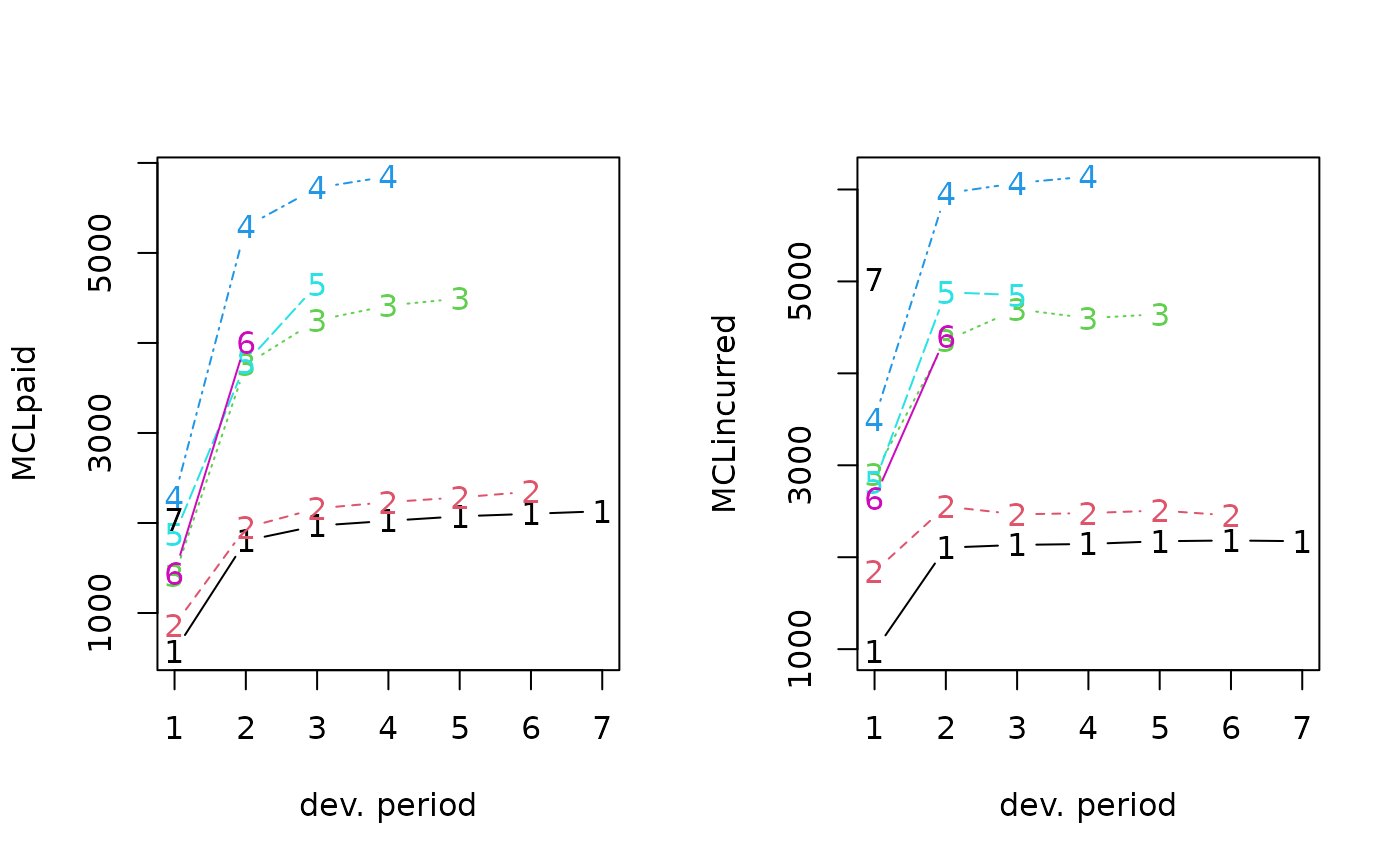 par(op)
# Following the example in Quarg's (2004) paper:
MCL <- MunichChainLadder(MCLpaid, MCLincurred, est.sigmaP=0.1, est.sigmaI=0.1)
MCL
#> MunichChainLadder(Paid = MCLpaid, Incurred = MCLincurred, est.sigmaP = 0.1,
#> est.sigmaI = 0.1)
#>
#> Latest Paid Latest Incurred Latest P/I Ratio Ult. Paid Ult. Incurred
#> 1 2,131 2,174 0.980 2,131 2,174
#> 2 2,348 2,454 0.957 2,383 2,444
#> 3 4,494 4,644 0.968 4,597 4,629
#> 4 5,850 6,142 0.952 6,119 6,176
#> 5 4,648 4,852 0.958 4,937 4,950
#> 6 4,010 4,406 0.910 4,656 4,665
#> 7 2,044 5,022 0.407 7,549 7,650
#> Ult. P/I Ratio
#> 1 0.980
#> 2 0.975
#> 3 0.993
#> 4 0.991
#> 5 0.997
#> 6 0.998
#> 7 0.987
#>
#> Totals
#> Paid Incurred P/I Ratio
#> Latest: 25,525 29,694 0.86
#> Ultimate: 32,371 32,688 0.99
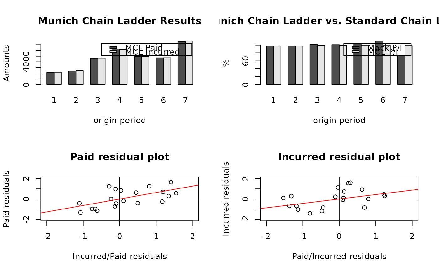
plot(MCL)
par(op)
# Following the example in Quarg's (2004) paper:
MCL <- MunichChainLadder(MCLpaid, MCLincurred, est.sigmaP=0.1, est.sigmaI=0.1)
MCL
#> MunichChainLadder(Paid = MCLpaid, Incurred = MCLincurred, est.sigmaP = 0.1,
#> est.sigmaI = 0.1)
#>
#> Latest Paid Latest Incurred Latest P/I Ratio Ult. Paid Ult. Incurred
#> 1 2,131 2,174 0.980 2,131 2,174
#> 2 2,348 2,454 0.957 2,383 2,444
#> 3 4,494 4,644 0.968 4,597 4,629
#> 4 5,850 6,142 0.952 6,119 6,176
#> 5 4,648 4,852 0.958 4,937 4,950
#> 6 4,010 4,406 0.910 4,656 4,665
#> 7 2,044 5,022 0.407 7,549 7,650
#> Ult. P/I Ratio
#> 1 0.980
#> 2 0.975
#> 3 0.993
#> 4 0.991
#> 5 0.997
#> 6 0.998
#> 7 0.987
#>
#> Totals
#> Paid Incurred P/I Ratio
#> Latest: 25,525 29,694 0.86
#> Ultimate: 32,371 32,688 0.99
plot(MCL)
 # You can access the standard chain-ladder (Mack) output via
MCL$MackPaid
#> MackChainLadder(Triangle = Paid, weights = weights, est.sigma = est.sigmaP,
#> tail = tailP)
#>
#> Latest Dev.To.Date Ultimate IBNR Mack.S.E CV(IBNR)
#> 1 2,131 1.000 2,131 0.0 0.00 NaN
#> 2 2,348 0.986 2,380 32.4 7.05 0.218
#> 3 4,494 0.966 4,652 158.2 47.92 0.303
#> 4 5,850 0.946 6,182 331.6 63.52 0.192
#> 5 4,648 0.919 5,056 407.6 67.54 0.166
#> 6 4,010 0.813 4,934 924.1 289.09 0.313
#> 7 2,044 0.334 6,128 4,084.3 897.13 0.220
#>
#> Totals
#> Latest: 25,525.00
#> Dev: 0.81
#> Ultimate: 31,463.21
#> IBNR: 5,938.21
#> Mack.S.E 987.23
#> CV(IBNR): 0.17
MCL$MackIncurred
#> MackChainLadder(Triangle = Incurred, weights = weights, est.sigma = est.sigmaI,
#> tail = tailI)
#>
#> Latest Dev.To.Date Ultimate IBNR Mack.S.E CV(IBNR)
#> 1 2,174 1.000 2,174 0.0 0.00 NaN
#> 2 2,454 1.004 2,445 -9.0 7.22 -0.803
#> 3 4,644 1.014 4,582 -62.5 83.30 -1.333
#> 4 6,142 1.003 6,126 -15.6 104.85 -6.705
#> 5 4,852 1.003 4,839 -13.0 118.50 -9.128
#> 6 4,406 0.984 4,476 70.1 217.45 3.101
#> 7 5,022 0.596 8,429 3,406.8 874.91 0.257
#>
#> Totals
#> Latest: 29,694.00
#> Dev: 0.90
#> Ultimate: 33,070.85
#> IBNR: 3,376.85
#> Mack.S.E 994.23
#> CV(IBNR): 0.29
# Input triangles section 3.3.1
MCL$Paid
#> dev
#> origin 1 2 3 4 5 6 7
#> 1 576 1804 1970 2024 2074 2102 2131
#> 2 866 1948 2162 2232 2284 2348 NA
#> 3 1412 3758 4252 4416 4494 NA NA
#> 4 2286 5292 5724 5850 NA NA NA
#> 5 1868 3778 4648 NA NA NA NA
#> 6 1442 4010 NA NA NA NA NA
#> 7 2044 NA NA NA NA NA NA
MCL$Incurred
#> dev
#> origin 1 2 3 4 5 6 7
#> 1 978 2104 2134 2144 2174 2182 2174
#> 2 1844 2552 2466 2480 2508 2454 NA
#> 3 2904 4354 4698 4600 4644 NA NA
#> 4 3502 5958 6070 6142 NA NA NA
#> 5 2812 4882 4852 NA NA NA NA
#> 6 2642 4406 NA NA NA NA NA
#> 7 5022 NA NA NA NA NA NA
# Parameters from section 3.3.2
# Standard chain-ladder age-to-age factors
MCL$MackPaid$f
#> [1] 2.436686 1.131242 1.029345 1.020756 1.021111 1.013796 1.000000
MCL$MackIncurred$f
#> [1] 1.6520910 1.0186398 0.9998699 1.0110581 0.9901751 0.9963336 1.0000000
MCL$MackPaid$sigma
#> [1] 13.4559310 3.6656420 0.4819578 0.2100029 0.4787308 0.1000000
MCL$MackIncurred$sigma
#> [1] 9.7273990 2.5444838 1.0040570 0.1200991 0.8603340 0.1000000
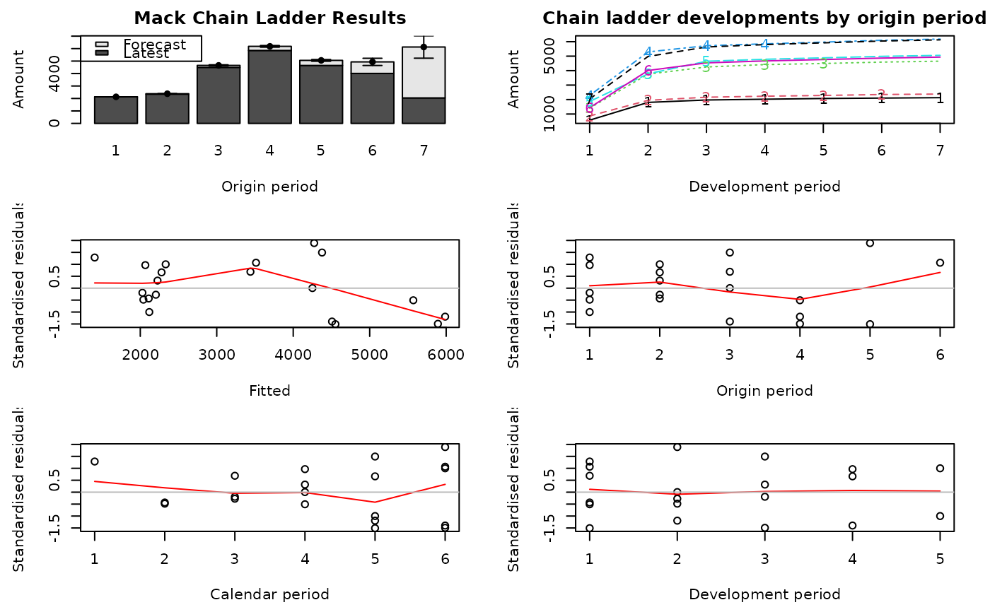
# Check Mack's assumptions graphically
plot(MCL$MackPaid)
# You can access the standard chain-ladder (Mack) output via
MCL$MackPaid
#> MackChainLadder(Triangle = Paid, weights = weights, est.sigma = est.sigmaP,
#> tail = tailP)
#>
#> Latest Dev.To.Date Ultimate IBNR Mack.S.E CV(IBNR)
#> 1 2,131 1.000 2,131 0.0 0.00 NaN
#> 2 2,348 0.986 2,380 32.4 7.05 0.218
#> 3 4,494 0.966 4,652 158.2 47.92 0.303
#> 4 5,850 0.946 6,182 331.6 63.52 0.192
#> 5 4,648 0.919 5,056 407.6 67.54 0.166
#> 6 4,010 0.813 4,934 924.1 289.09 0.313
#> 7 2,044 0.334 6,128 4,084.3 897.13 0.220
#>
#> Totals
#> Latest: 25,525.00
#> Dev: 0.81
#> Ultimate: 31,463.21
#> IBNR: 5,938.21
#> Mack.S.E 987.23
#> CV(IBNR): 0.17
MCL$MackIncurred
#> MackChainLadder(Triangle = Incurred, weights = weights, est.sigma = est.sigmaI,
#> tail = tailI)
#>
#> Latest Dev.To.Date Ultimate IBNR Mack.S.E CV(IBNR)
#> 1 2,174 1.000 2,174 0.0 0.00 NaN
#> 2 2,454 1.004 2,445 -9.0 7.22 -0.803
#> 3 4,644 1.014 4,582 -62.5 83.30 -1.333
#> 4 6,142 1.003 6,126 -15.6 104.85 -6.705
#> 5 4,852 1.003 4,839 -13.0 118.50 -9.128
#> 6 4,406 0.984 4,476 70.1 217.45 3.101
#> 7 5,022 0.596 8,429 3,406.8 874.91 0.257
#>
#> Totals
#> Latest: 29,694.00
#> Dev: 0.90
#> Ultimate: 33,070.85
#> IBNR: 3,376.85
#> Mack.S.E 994.23
#> CV(IBNR): 0.29
# Input triangles section 3.3.1
MCL$Paid
#> dev
#> origin 1 2 3 4 5 6 7
#> 1 576 1804 1970 2024 2074 2102 2131
#> 2 866 1948 2162 2232 2284 2348 NA
#> 3 1412 3758 4252 4416 4494 NA NA
#> 4 2286 5292 5724 5850 NA NA NA
#> 5 1868 3778 4648 NA NA NA NA
#> 6 1442 4010 NA NA NA NA NA
#> 7 2044 NA NA NA NA NA NA
MCL$Incurred
#> dev
#> origin 1 2 3 4 5 6 7
#> 1 978 2104 2134 2144 2174 2182 2174
#> 2 1844 2552 2466 2480 2508 2454 NA
#> 3 2904 4354 4698 4600 4644 NA NA
#> 4 3502 5958 6070 6142 NA NA NA
#> 5 2812 4882 4852 NA NA NA NA
#> 6 2642 4406 NA NA NA NA NA
#> 7 5022 NA NA NA NA NA NA
# Parameters from section 3.3.2
# Standard chain-ladder age-to-age factors
MCL$MackPaid$f
#> [1] 2.436686 1.131242 1.029345 1.020756 1.021111 1.013796 1.000000
MCL$MackIncurred$f
#> [1] 1.6520910 1.0186398 0.9998699 1.0110581 0.9901751 0.9963336 1.0000000
MCL$MackPaid$sigma
#> [1] 13.4559310 3.6656420 0.4819578 0.2100029 0.4787308 0.1000000
MCL$MackIncurred$sigma
#> [1] 9.7273990 2.5444838 1.0040570 0.1200991 0.8603340 0.1000000
# Check Mack's assumptions graphically
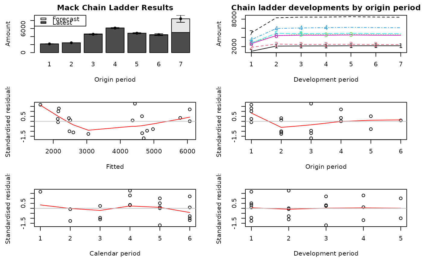
plot(MCL$MackPaid)
 plot(MCL$MackIncurred)
 MCL$q.f
#> [1] 0.5325822 0.8488621 0.9275964 0.9450735 0.9491744 0.9598792 0.9802208
MCL$rhoP.sigma
#> [1] 14.9430129 4.9899464 2.1665565 1.6186098 1.7910011 0.2359799 0.1966189
MCL$rhoI.sigma
#> [1] 5.7107795 3.8192859 1.9184007 1.4606629 1.6370399 0.2219648 0.2494577
MCL$PaidResiduals
#> [1] 1.240062341 -0.409542454 0.627731906 -0.432520662 -1.330415661
#> [6] 0.971284236 NA -0.454493935 -0.257500458 0.003519297
#> [11] -0.984526495 1.660669736 NA NA -0.178096214
#> [16] 0.292551156 1.248117471 -1.151042283 NA NA
#> [21] NA 0.845586577 0.571652630 -0.978875177 NA
#> [26] NA NA NA -0.723943106 0.689859681
#> [31] NA NA NA NA NA
#> [36] NA NA NA NA NA
#> [41] NA NA NA NA NA
#> [46] NA NA NA NA
MCL$IncurredResiduals
#> [1] 1.605020358 -1.183723533 -0.846383581 0.299450714 0.458137992
#> [6] 0.082352480 NA -0.078980622 -1.039118036 1.565493903
#> [11] 0.004806834 -0.680589085 NA NA 0.221585430
#> [16] 0.287221014 -1.415119918 0.930505026 NA NA
#> [21] NA 1.131348046 0.096288253 -0.843077797 NA
#> [26] NA NA NA 0.731893789 -0.681418728
#> [31] NA NA NA NA NA
#> [36] NA NA NA NA NA
#> [41] NA NA NA NA NA
#> [46] NA NA NA NA
MCL$QinverseResiduals
#> [1] -0.28866099 0.49565517 0.45015637 -1.10614730 -1.07679458 -0.11554182
#> [7] NA -0.10001795 1.16766593 -0.23897922 -0.76095980 1.40633581
#> [13] NA NA 0.10639977 1.34252842 0.80771329 -0.61487164
#> [19] NA NA NA 0.03251491 1.54674415 -0.67544873
#> [25] NA NA NA NA -0.13556094 1.18814416
#> [31] NA NA NA NA NA NA
#> [37] NA NA NA NA NA NA
#> [43] NA NA NA NA NA NA
#> [49] NA
MCL$QResiduals
#> [1] 0.30871615 -0.47335565 -0.43743334 1.24543896 1.22304681 0.11895559
#> [7] NA 0.10271271 -1.13141939 0.24623239 0.79537557 -1.37205649
#> [13] NA NA -0.10709430 -1.31687503 -0.80498376 0.62550343
#> [19] NA NA NA -0.03308516 -1.53672981 0.69308386
#> [25] NA NA NA NA 0.13749654 -1.17743245
#> [31] NA NA NA NA NA NA
#> [37] NA NA NA NA NA NA
#> [43] NA NA NA NA NA NA
#> [49] NA
MCL$lambdaP
#>
#> Call:
#> lm(formula = PaidResiduals ~ QinverseResiduals + 0)
#>
#> Coefficients:
#> QinverseResiduals
#> 0.636
#>
MCL$lambdaI
#>
#> Call:
#> lm(formula = IncurredResiduals ~ QResiduals + 0)
#>
#> Coefficients:
#> QResiduals
#> 0.4362
#>
# Section 3.3.3 Results
MCL$MCLPaid
#> 1 2 3 4 5 6
#> 1 576 1804.00 1970.000 2024.000 2074.000 2102.000 2131.000
#> 2 866 1948.00 2162.000 2232.000 2284.000 2348.000 2382.512
#> 3 1412 3758.00 4252.000 4416.000 4494.000 4573.461 4597.066
#> 4 2286 5292.00 5724.000 5850.000 5967.465 6080.613 6119.269
#> 5 1868 3778.00 4648.000 4761.928 4848.086 4922.643 4937.412
#> 6 1442 4010.00 4387.718 4493.324 4573.894 4642.893 4655.543
#> 7 2044 5658.75 6944.326 7176.571 7329.680 7485.196 7548.518
MCL$MCLIncurred
#> 1 2 3 4 5 6
#> 1 978 2104.00 2134.000 2144.000 2174.000 2182.000 2174.000
#> 2 1844 2552.00 2466.000 2480.000 2508.000 2454.000 2443.520
#> 3 2904 4354.00 4698.000 4600.000 4644.000 4618.095 4628.803
#> 4 3502 5958.00 6070.000 6142.000 6211.546 6166.937 6175.985
#> 5 2812 4882.00 4852.000 4884.997 4944.225 4931.215 4950.330
#> 6 2642 4406.00 4566.563 4600.621 4656.710 4646.230 4665.171
#> 7 5022 7828.26 7687.543 7643.941 7726.764 7649.849 7649.759
MCL$q.f
#> [1] 0.5325822 0.8488621 0.9275964 0.9450735 0.9491744 0.9598792 0.9802208
MCL$rhoP.sigma
#> [1] 14.9430129 4.9899464 2.1665565 1.6186098 1.7910011 0.2359799 0.1966189
MCL$rhoI.sigma
#> [1] 5.7107795 3.8192859 1.9184007 1.4606629 1.6370399 0.2219648 0.2494577
MCL$PaidResiduals
#> [1] 1.240062341 -0.409542454 0.627731906 -0.432520662 -1.330415661
#> [6] 0.971284236 NA -0.454493935 -0.257500458 0.003519297
#> [11] -0.984526495 1.660669736 NA NA -0.178096214
#> [16] 0.292551156 1.248117471 -1.151042283 NA NA
#> [21] NA 0.845586577 0.571652630 -0.978875177 NA
#> [26] NA NA NA -0.723943106 0.689859681
#> [31] NA NA NA NA NA
#> [36] NA NA NA NA NA
#> [41] NA NA NA NA NA
#> [46] NA NA NA NA
MCL$IncurredResiduals
#> [1] 1.605020358 -1.183723533 -0.846383581 0.299450714 0.458137992
#> [6] 0.082352480 NA -0.078980622 -1.039118036 1.565493903
#> [11] 0.004806834 -0.680589085 NA NA 0.221585430
#> [16] 0.287221014 -1.415119918 0.930505026 NA NA
#> [21] NA 1.131348046 0.096288253 -0.843077797 NA
#> [26] NA NA NA 0.731893789 -0.681418728
#> [31] NA NA NA NA NA
#> [36] NA NA NA NA NA
#> [41] NA NA NA NA NA
#> [46] NA NA NA NA
MCL$QinverseResiduals
#> [1] -0.28866099 0.49565517 0.45015637 -1.10614730 -1.07679458 -0.11554182
#> [7] NA -0.10001795 1.16766593 -0.23897922 -0.76095980 1.40633581
#> [13] NA NA 0.10639977 1.34252842 0.80771329 -0.61487164
#> [19] NA NA NA 0.03251491 1.54674415 -0.67544873
#> [25] NA NA NA NA -0.13556094 1.18814416
#> [31] NA NA NA NA NA NA
#> [37] NA NA NA NA NA NA
#> [43] NA NA NA NA NA NA
#> [49] NA
MCL$QResiduals
#> [1] 0.30871615 -0.47335565 -0.43743334 1.24543896 1.22304681 0.11895559
#> [7] NA 0.10271271 -1.13141939 0.24623239 0.79537557 -1.37205649
#> [13] NA NA -0.10709430 -1.31687503 -0.80498376 0.62550343
#> [19] NA NA NA -0.03308516 -1.53672981 0.69308386
#> [25] NA NA NA NA 0.13749654 -1.17743245
#> [31] NA NA NA NA NA NA
#> [37] NA NA NA NA NA NA
#> [43] NA NA NA NA NA NA
#> [49] NA
MCL$lambdaP
#>
#> Call:
#> lm(formula = PaidResiduals ~ QinverseResiduals + 0)
#>
#> Coefficients:
#> QinverseResiduals
#> 0.636
#>
MCL$lambdaI
#>
#> Call:
#> lm(formula = IncurredResiduals ~ QResiduals + 0)
#>
#> Coefficients:
#> QResiduals
#> 0.4362
#>
# Section 3.3.3 Results
MCL$MCLPaid
#> 1 2 3 4 5 6
#> 1 576 1804.00 1970.000 2024.000 2074.000 2102.000 2131.000
#> 2 866 1948.00 2162.000 2232.000 2284.000 2348.000 2382.512
#> 3 1412 3758.00 4252.000 4416.000 4494.000 4573.461 4597.066
#> 4 2286 5292.00 5724.000 5850.000 5967.465 6080.613 6119.269
#> 5 1868 3778.00 4648.000 4761.928 4848.086 4922.643 4937.412
#> 6 1442 4010.00 4387.718 4493.324 4573.894 4642.893 4655.543
#> 7 2044 5658.75 6944.326 7176.571 7329.680 7485.196 7548.518
MCL$MCLIncurred
#> 1 2 3 4 5 6
#> 1 978 2104.00 2134.000 2144.000 2174.000 2182.000 2174.000
#> 2 1844 2552.00 2466.000 2480.000 2508.000 2454.000 2443.520
#> 3 2904 4354.00 4698.000 4600.000 4644.000 4618.095 4628.803
#> 4 3502 5958.00 6070.000 6142.000 6211.546 6166.937 6175.985
#> 5 2812 4882.00 4852.000 4884.997 4944.225 4931.215 4950.330
#> 6 2642 4406.00 4566.563 4600.621 4656.710 4646.230 4665.171
#> 7 5022 7828.26 7687.543 7643.941 7726.764 7649.849 7649.759