Quarterly run off triangle of accumulated claims data
qpaid.rdSample data to demonstrate how to work with triangles with a higher development period frequency than origin period frequency
Examples
dim(qpaid)
#> [1] 12 45
dim(qincurred)
#> [1] 12 45
op=par(mfrow=c(1,2))
ymax <- max(c(qpaid,qincurred),na.rm=TRUE)*1.05
matplot(t(qpaid), type="l", main="Paid development",
xlab="Dev. quarter", ylab="$", ylim=c(0,ymax))
matplot(t(qincurred), type="l", main="Incurred development",
xlab="Dev. quarter", ylab="$", ylim=c(0,ymax))
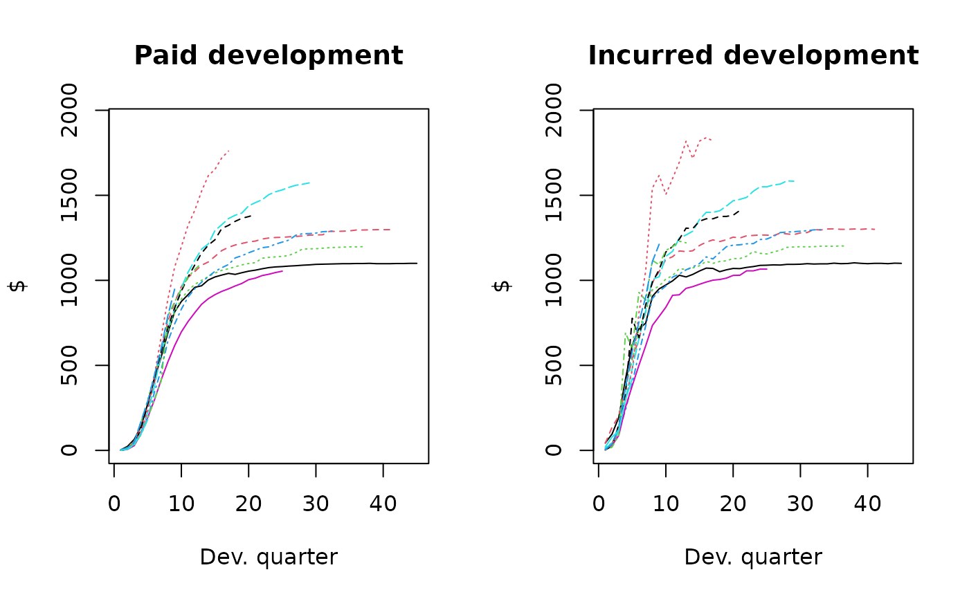 par(op)
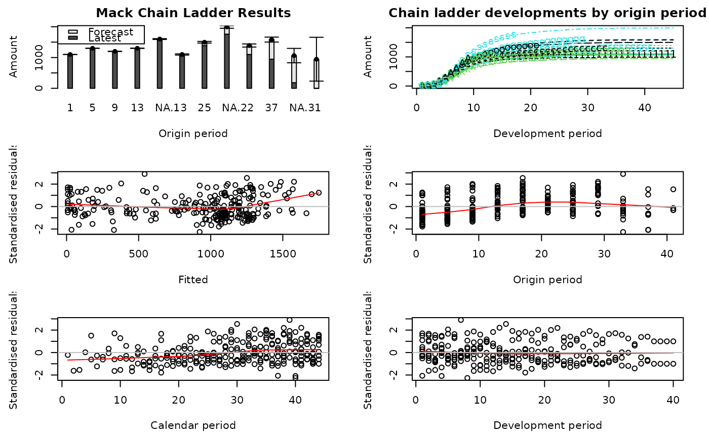
## MackChainLadder expects a quadratic matrix so let's expand
## the triangle to a quarterly origin period.
n <- ncol(qpaid)
Paid <- matrix(NA, n, n)
Paid[seq(1,n,4),] <- qpaid
M <- MackChainLadder(Paid)
#> Warning: Information: essentially no variation in development data for period(s):
#> '39-40', '40-41'
plot(M)
par(op)
## MackChainLadder expects a quadratic matrix so let's expand
## the triangle to a quarterly origin period.
n <- ncol(qpaid)
Paid <- matrix(NA, n, n)
Paid[seq(1,n,4),] <- qpaid
M <- MackChainLadder(Paid)
#> Warning: Information: essentially no variation in development data for period(s):
#> '39-40', '40-41'
plot(M)
 # We expand the incurred triangle in the same way
Incurred <- matrix(NA, n, n)
Incurred[seq(1,n,4),] <- qincurred
# With the expanded triangles we can apply MunichChainLadder
MunichChainLadder(Paid, Incurred)
#> Warning: Information: essentially no variation in development data for period(s):
#> '39-40', '40-41'
#> MunichChainLadder(Paid = Paid, Incurred = Incurred)
#>
#> Latest Paid Latest Incurred Latest P/I Ratio Ult. Paid Ult. Incurred
#> 1 1,100 1,100 1.0000 1,100 1,100
#> 5 1,298 1,300 0.9985 1,300 1,300
#> 9 1,198 1,200 0.9983 1,201 1,201
#> 13 1,293 1,298 0.9961 1,301 1,301
#> 17 1,573 1,583 0.9937 1,601 1,601
#> 21 1,054 1,066 0.9887 1,100 1,100
#> 25 1,387 1,411 0.9830 1,498 1,498
#> 29 1,760 1,820 0.9670 1,995 1,995
#> 33 1,100 1,221 0.9009 1,398 1,397
#> 37 948 1,212 0.7822 1,590 1,590
#> 41 183 422 0.4336 1,086 1,086
#> 45 1 13 0.0769 1,073 1,073
#> Ult. P/I Ratio
#> 1 1
#> 5 1
#> 9 1
#> 13 1
#> 17 1
#> 21 1
#> 25 1
#> 29 1
#> 33 1
#> 37 1
#> 41 1
#> 45 1
#>
#> Totals
#> Paid Incurred P/I Ratio
#> Latest: 12,895 13,646 0.94
#> Ultimate: 16,243 16,242 1.00
# In the same way we can apply BootChainLadder
# We reduce the size of bootstrap replicates R
# from the default of 999 to 99 purely to reduce run time.
BootChainLadder(Paid, R=99)
#> BootChainLadder(Triangle = Paid, R = 99)
#>
#> Latest Mean Ultimate Mean IBNR IBNR.S.E IBNR 75% IBNR 95%
#> 1 1,100 1,100 0.00 0.00 0.00 0.0
#> 5 1,298 1,301 2.60 4.26 4.59 11.0
#> 9 1,198 1,201 2.59 4.54 5.10 10.9
#> 13 1,293 1,301 8.48 6.99 12.24 19.2
#> 17 1,573 1,602 28.67 11.12 35.09 46.0
#> 21 1,054 1,100 46.48 11.01 54.70 64.9
#> 25 1,387 1,495 107.95 18.83 119.96 138.5
#> 29 1,760 1,996 236.14 28.05 252.68 279.6
#> 33 1,100 1,392 292.37 33.20 312.90 348.2
#> 37 948 1,579 631.45 61.51 678.66 729.6
#> 41 183 1,049 866.08 165.54 950.38 1,159.0
#> 45 1 2,205 2,204.21 17,541.52 1,628.87 4,764.8
#>
#> Totals
#> Latest: 12,895
#> Mean Ultimate: 17,322
#> Mean IBNR: 4,427
#> IBNR.S.E 17,509
#> Total IBNR 75%: 3,997
#> Total IBNR 95%: 7,087
# We expand the incurred triangle in the same way
Incurred <- matrix(NA, n, n)
Incurred[seq(1,n,4),] <- qincurred
# With the expanded triangles we can apply MunichChainLadder
MunichChainLadder(Paid, Incurred)
#> Warning: Information: essentially no variation in development data for period(s):
#> '39-40', '40-41'
#> MunichChainLadder(Paid = Paid, Incurred = Incurred)
#>
#> Latest Paid Latest Incurred Latest P/I Ratio Ult. Paid Ult. Incurred
#> 1 1,100 1,100 1.0000 1,100 1,100
#> 5 1,298 1,300 0.9985 1,300 1,300
#> 9 1,198 1,200 0.9983 1,201 1,201
#> 13 1,293 1,298 0.9961 1,301 1,301
#> 17 1,573 1,583 0.9937 1,601 1,601
#> 21 1,054 1,066 0.9887 1,100 1,100
#> 25 1,387 1,411 0.9830 1,498 1,498
#> 29 1,760 1,820 0.9670 1,995 1,995
#> 33 1,100 1,221 0.9009 1,398 1,397
#> 37 948 1,212 0.7822 1,590 1,590
#> 41 183 422 0.4336 1,086 1,086
#> 45 1 13 0.0769 1,073 1,073
#> Ult. P/I Ratio
#> 1 1
#> 5 1
#> 9 1
#> 13 1
#> 17 1
#> 21 1
#> 25 1
#> 29 1
#> 33 1
#> 37 1
#> 41 1
#> 45 1
#>
#> Totals
#> Paid Incurred P/I Ratio
#> Latest: 12,895 13,646 0.94
#> Ultimate: 16,243 16,242 1.00
# In the same way we can apply BootChainLadder
# We reduce the size of bootstrap replicates R
# from the default of 999 to 99 purely to reduce run time.
BootChainLadder(Paid, R=99)
#> BootChainLadder(Triangle = Paid, R = 99)
#>
#> Latest Mean Ultimate Mean IBNR IBNR.S.E IBNR 75% IBNR 95%
#> 1 1,100 1,100 0.00 0.00 0.00 0.0
#> 5 1,298 1,301 2.60 4.26 4.59 11.0
#> 9 1,198 1,201 2.59 4.54 5.10 10.9
#> 13 1,293 1,301 8.48 6.99 12.24 19.2
#> 17 1,573 1,602 28.67 11.12 35.09 46.0
#> 21 1,054 1,100 46.48 11.01 54.70 64.9
#> 25 1,387 1,495 107.95 18.83 119.96 138.5
#> 29 1,760 1,996 236.14 28.05 252.68 279.6
#> 33 1,100 1,392 292.37 33.20 312.90 348.2
#> 37 948 1,579 631.45 61.51 678.66 729.6
#> 41 183 1,049 866.08 165.54 950.38 1,159.0
#> 45 1 2,205 2,204.21 17,541.52 1,628.87 4,764.8
#>
#> Totals
#> Latest: 12,895
#> Mean Ultimate: 17,322
#> Mean IBNR: 4,427
#> IBNR.S.E 17,509
#> Total IBNR 75%: 3,997
#> Total IBNR 95%: 7,087