GLM-based Reserving Model

This function implements loss reserving models within the generalized linear model framework. It takes accident year and development lag as mean predictors in estimating the ultimate loss reserves, and provides both analytical and bootstrapping methods to compute the associated prediction errors. The bootstrapping approach also generates the full predictive distribution for loss reserves.

Usage

glmReserve(triangle, var.power = 1, link.power = 0, cum = TRUE, 
      mse.method = c("formula", "bootstrap"),  nsim = 1000, nb = FALSE, ...)

Arguments

triangle

An object of class triangle.

var.power

The index (p) of the power variance function \(V(\mu)=\mu^p\). Default to p = 1, which is the over-dispersed Poisson model. If NULL, it will be assumed to be in (1, 2) and estimated using the cplm package. See tweedie.

link.power

The index of power link function. The default link.power = 0 produces a log link. See tweedie.

cum

A logical value indicating whether the input triangle is on the cumulative or the incremental scale. If TRUE, then triangle is assumed to be on the cumulative scale, and it will be converted to incremental losses internally before a GLM is fitted.

mse.method

A character indicating whether the prediction error should be computed analytically (mse.method = "formula") or via bootstrapping (mse.method = "bootstrap"). Partial match is supported.

nsim

Number of simulations to be performed in the bootstrapping, with a default value of 1000.

nb

Whether the negative binomial distribution is used. If true, the arguments var.power and link.power are ignored and a negative binomial GLM is fitted using glm.nb.

...

Arguments to be passed onto the function glm or cpglm such as contrasts or control. It is important that offset and weight should not be specified. Otherwise, an error will be reported and the program will quit.

Details

This function takes an insurance loss triangle, converts it to incremental losses internally if necessary, transforms it to the long format (see as.data.frame) and fits the resulting loss data with a generalized linear model where the mean structure includes both the accident year and the development lag effects. The distributions allowed are the exponential family that admits a power variance function, that is, \(V(\mu)=\mu^p\). This subclass of distributions is usually called the Tweedie distribution and includes many commonly used distributions as special cases.

This function does not allow the user to specify the GLM options through the usual family argument, but instead, it uses the tweedie family internally and takes two arguments, var.power and link.power, through which the user still has full control of the distribution forms and link functions. The argument var.power determines which specific distribution is to be used, and link.power determines the form of the link function.

When the Tweedie compound Poisson distribution 1 < p < 2 is to be used, the user has the option to specify var.power = NULL, where the variance power p will be estimated from the data using the cplm package. The bcplm function in the cplm package also has an example for the Bayesian compound Poisson loss reserving model. See details in tweedie, cpglm and bcplm.

glmReserve allows certain measures of exposures to be used in an offset term in the underlying GLM. To do this, the user should not use the usual offset argument in glm. Instead, one specifies the exposure measure for each accident year through the exposure attribute of triangle. Make sure that these exposures are in the original scale (no log transformations for example). If the vector is named, make sure the names coincide with the rownames/origin of the triangle. If the vector is unnamed, make sure the exposures are in the order consistent with the accident years, and the character rownames of the Triangle must be convertible to numeric. If the exposure attribute is not NULL, the glmReserve function will use these exposures, link-function-transformed, in the offset term of the GLM. For example, if the link function is log, then the log of the exposure is used as the offset, not the original exposure. See the examples below. Moreover, the user MUST NOT supply the typical offset or weight as arguments in the list of additional arguments .... offset should be specified as above, while weight is not implemented (due to prediction reasons).

Two methods are available to assess the prediction error of the estimated loss reserves. One is using the analytical formula (mse.method = "formula") derived from the first-order Taylor approximation. The other is using bootstrapping (mse.method = "bootstrap") that reconstructs the triangle nsim times by sampling with replacement from the GLM (Pearson) residuals. Each time a new triangle is formed, GLM is fitted and corresponding loss reserves are generated. Based on these predicted mean loss reserves, and the model assumption about the distribution forms, realizations of the predicted values are generated via the rtweedie function. Prediction errors as well as other uncertainty measures such as quantiles and predictive intervals can be calculated based on these samples.

Note

The use of GLM in insurance loss reserving has many compelling aspects, e.g.,

• when over-dispersed Poisson model is used, it reproduces the estimates from Chain Ladder;

• it provides a more coherent modeling framework than the Mack method;

• all the relevant established statistical theory can be directly applied to perform hypothesis testing and diagnostic checking;

However, the user should be cautious of some of the key assumptions that underlie the GLM model, in order to determine whether this model is appropriate for the problem considered:

• the GLM model assumes no tail development, and it only projects losses to the latest time point of the observed data. To use a model that enables tail extrapolation, please consider the growth curve model ClarkLDF or ClarkCapeCod;

• the model assumes that each incremental loss is independent of all the others. This assumption may not be valid in that cells from the same calendar year are usually correlated due to inflation or business operating factors;

• the model tends to be over-parameterized, which may lead to inferior predictive performance.

To solve these potential problems, many variants of the current basic GLM model have been proposed in the actuarial literature. Some of these may be included in the future release.

Support of the negative binomial GLM was added since version 0.2.3.

Value

The output is an object of class "glmReserve" that has the following components:

call

the matched call.

summary

A data frame containing the predicted loss reserve statistics. Similar to the summary statistics from MackChainLadder.

Triangle

The input triangle.

FullTriangle

The completed triangle, where empty cells in the original triangle are filled with model predictions.

model

The fitted GLM, a class of "glm" or "cpglm". It is most convenient to work with this component when model fit information is wanted.

sims.par

a matrix of the simulated parameter values in the bootstrapping.

sims.reserve.mean

a matrix of the simulated mean loss reserves (without the process variance) for each year in the bootstrapping.

sims.par

a matrix of the simulated realizations of the loss reserves (with the process variance) for each year in the bootstrapping. This can be used to summarize the predictive uncertainty of the loss reserves.

References

England P. and Verrall R. (1999). Analytic and bootstrap estimates of prediction errors in claims reserving. Insurance: Mathematics and Economics, 25, 281-293.

Author

Wayne Zhang actuary_zhang@hotmail.com

See also

See also glm, glm.nb, tweedie, cpglm and MackChainLadder.

Examples

data(GenIns)
GenIns <- GenIns / 1000

# over-dispersed Poisson: reproduce ChainLadder estimates
(fit1 <- glmReserve(GenIns))
#>          Latest Dev.To.Date  Ultimate  IBNR       S.E        CV
#> 2      5339.085  0.98251776  5434.085    95  110.0999 1.1589460
#> 3      4909.315  0.91262828  5379.315   470  216.0434 0.4596668
#> 4      4588.268  0.86599394  5298.268   710  260.8721 0.3674255
#> 5      3873.311  0.79725464  4858.311   985  303.5500 0.3081726
#> 6      3691.712  0.72234788  5110.712  1419  375.0139 0.2642804
#> 7      3483.130  0.61527116  5661.130  2178  495.3780 0.2274463
#> 8      2864.498  0.42221223  6784.498  3920  789.9611 0.2015207
#> 9      1363.294  0.24162052  5642.294  4279 1046.5138 0.2445697
#> 10      344.014  0.06921791  4970.014  4626 1980.1014 0.4280375
#> total 30456.627  0.61982291 49137.627 18681 2945.6609 0.1576822
summary(fit1, type = "model")   # extract the underlying glm
#> 
#> Call:
#> glm(formula = value ~ factor(origin) + factor(dev), family = fam, 
#>     data = ldaFit, offset = offset)
#> 
#> Coefficients:
#>                   Estimate Std. Error t value Pr(>|t|)    
#> (Intercept)       5.598649   0.172924  32.376  < 2e-16 ***
#> factor(origin)2   0.331272   0.153537   2.158  0.03771 *  
#> factor(origin)3   0.321119   0.157719   2.036  0.04916 *  
#> factor(origin)4   0.305960   0.160736   1.903  0.06499 .  
#> factor(origin)5   0.219316   0.167970   1.306  0.19994    
#> factor(origin)6   0.270077   0.170756   1.582  0.12247    
#> factor(origin)7   0.372208   0.174451   2.134  0.03976 *  
#> factor(origin)8   0.553333   0.186525   2.967  0.00532 ** 
#> factor(origin)9   0.368934   0.239181   1.542  0.13170    
#> factor(origin)10  0.242033   0.427562   0.566  0.57485    
#> factor(dev)2      0.912526   0.148850   6.131 4.65e-07 ***
#> factor(dev)3      0.958831   0.152569   6.285 2.90e-07 ***
#> factor(dev)4      1.025997   0.156883   6.540 1.33e-07 ***
#> factor(dev)5      0.435276   0.183914   2.367  0.02344 *  
#> factor(dev)6      0.080057   0.214770   0.373  0.71152    
#> factor(dev)7     -0.006381   0.238290  -0.027  0.97878    
#> factor(dev)8     -0.394452   0.310289  -1.271  0.21180    
#> factor(dev)9      0.009378   0.320249   0.029  0.97680    
#> factor(dev)10    -1.379907   0.896690  -1.539  0.13258    
#> ---
#> Signif. codes:  0 ‘***’ 0.001 ‘**’ 0.01 ‘*’ 0.05 ‘.’ 0.1 ‘ ’ 1
#> 
#> (Dispersion parameter for Tweedie family taken to be 52.60193)
#> 
#>     Null deviance: 10699  on 54  degrees of freedom
#> Residual deviance:  1903  on 36  degrees of freedom
#> AIC: NA
#> 
#> Number of Fisher Scoring iterations: 4
#> 

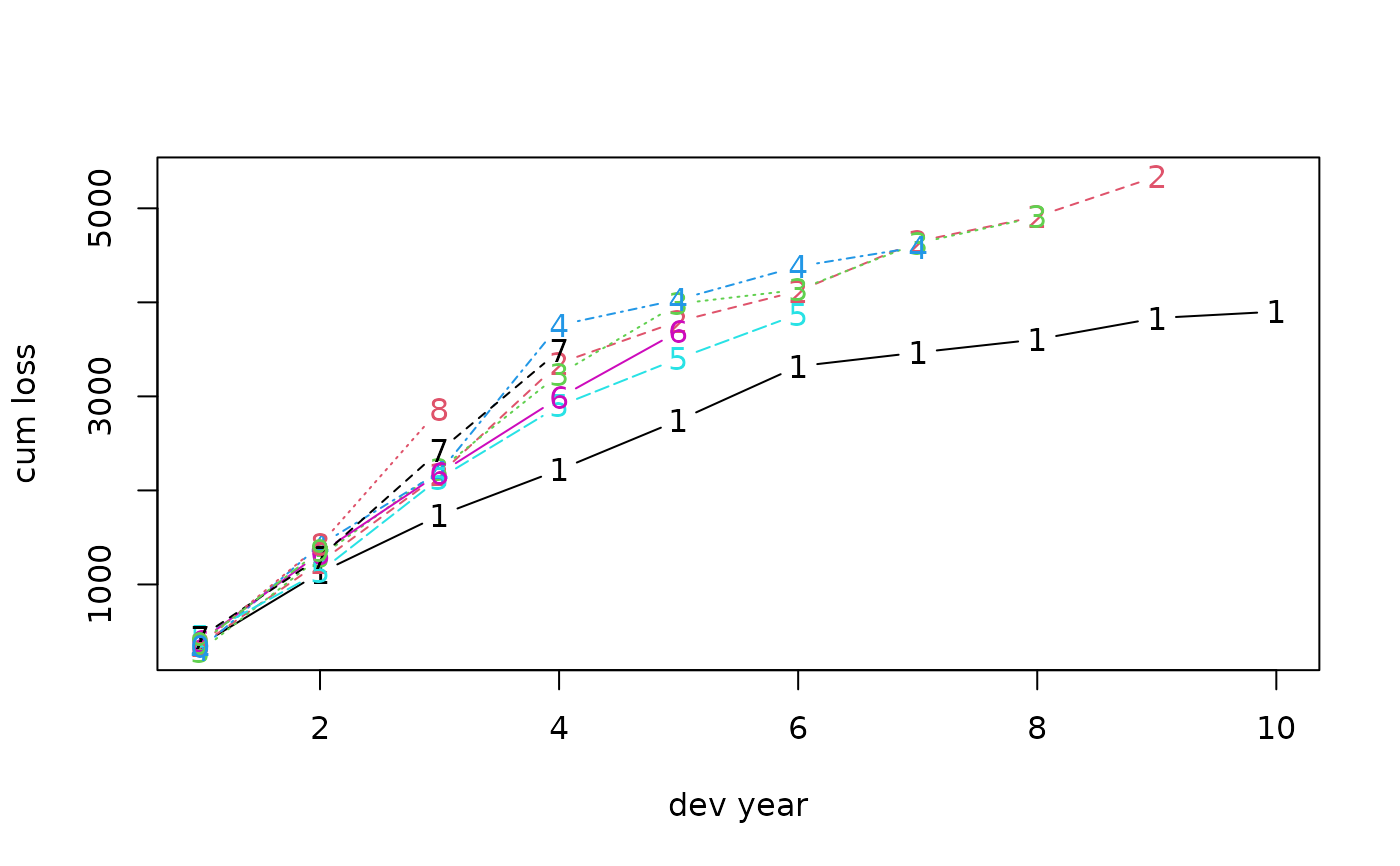
# which:
# 1 Original triangle 
# 2 Full triangle 
# 3 Reserve distribution
# 4 Residual plot
# 5 QQ-plot

# plot original triangle
plot(fit1, which = 1, xlab = "dev year", ylab = "cum loss")


# plot residuals 
plot(fit1, which = 4, xlab = "fitted values", ylab = "residuals")


# Gamma GLM:
(fit2 <- glmReserve(GenIns, var.power = 2))
#>          Latest Dev.To.Date  Ultimate  IBNR        S.E        CV
#> 2      5339.085  0.98287950  5432.085    93   45.16637 0.4856599
#> 3      4909.315  0.91654710  5356.315   447  160.55717 0.3591883
#> 4      4588.268  0.88248346  5199.268   611  177.62461 0.2907113
#> 5      3873.311  0.79610759  4865.311   992  254.47093 0.2565231
#> 6      3691.712  0.71757408  5144.712  1453  351.33426 0.2417992
#> 7      3483.130  0.61440292  5669.130  2186  526.28787 0.2407538
#> 8      2864.498  0.43870111  6529.498  3665  941.32225 0.2568410
#> 9      1363.294  0.24853618  5485.294  4122 1175.94587 0.2852853
#> 10      344.014  0.07078457  4860.014  4516 1667.39240 0.3692189
#> total 30456.627  0.62742025 48542.627 18086 2702.70978 0.1494366

# compound Poisson GLM (variance function estimated from the data):
(fit3 <- glmReserve(GenIns, var.power = NULL))
#>          Latest Dev.To.Date  Ultimate  IBNR        S.E        CV
#> 2      5339.085  0.98269860  5433.085    94   91.59865 0.9744537
#> 3      4909.315  0.91330741  5375.315   466  186.54619 0.4003137
#> 4      4588.268  0.86779562  5287.268   699  223.72322 0.3200618
#> 5      3873.311  0.79709058  4859.311   986  264.76238 0.2685217
#> 6      3691.712  0.72164188  5115.712  1424  333.24690 0.2340217
#> 7      3483.130  0.61505387  5663.130  2180  452.93426 0.2077680
#> 8      2864.498  0.42364843  6761.498  3897  754.58057 0.1936311
#> 9      1363.294  0.24230764  5626.294  4263 1019.45920 0.2391413
#> 10      344.014  0.06942745  4955.014  4611 1910.99069 0.4144417
#> total 30456.627  0.62058068 49077.627 18621 2831.45526 0.1520571

# Now suppose we have an exposure measure
# we can put it as an offset term in the model
# to do this, use the "exposure" attribute of the 'triangle'
expos <- (7 + 1:10 * 0.4) * 100
GenIns2 <- GenIns
attr(GenIns2, "exposure") <- expos
(fit4 <- glmReserve(GenIns2))
#>          Latest Dev.To.Date  Ultimate  IBNR       S.E        CV
#> 2      5339.085  0.98251776  5434.085    95  110.0999 1.1589460
#> 3      4909.315  0.91262828  5379.315   470  216.0434 0.4596668
#> 4      4588.268  0.86599394  5298.268   710  260.8721 0.3674255
#> 5      3873.311  0.79725464  4858.311   985  303.5500 0.3081726
#> 6      3691.712  0.72234788  5110.712  1419  375.0139 0.2642804
#> 7      3483.130  0.61527116  5661.130  2178  495.3780 0.2274463
#> 8      2864.498  0.42221223  6784.498  3920  789.9611 0.2015207
#> 9      1363.294  0.24162052  5642.294  4279 1046.5138 0.2445697
#> 10      344.014  0.06921791  4970.014  4626 1980.1014 0.4280375
#> total 30456.627  0.61982291 49137.627 18681 2945.6609 0.1576822
# If the triangle's rownames are not convertible to numeric,
# supply names to the exposures
GenIns3 <- GenIns2
rownames(GenIns3) <- paste0(2007:2016, "-01-01")
names(expos) <- rownames(GenIns3)
attr(GenIns3, "exposure") <- expos
(fit4b <- glmReserve(GenIns3))
#>               Latest Dev.To.Date  Ultimate  IBNR       S.E        CV
#> 2008-01-01  5339.085  0.98251776  5434.085    95  110.0999 1.1589460
#> 2009-01-01  4909.315  0.91262828  5379.315   470  216.0434 0.4596668
#> 2010-01-01  4588.268  0.86599394  5298.268   710  260.8721 0.3674255
#> 2011-01-01  3873.311  0.79725464  4858.311   985  303.5500 0.3081726
#> 2012-01-01  3691.712  0.72234788  5110.712  1419  375.0139 0.2642804
#> 2013-01-01  3483.130  0.61527116  5661.130  2178  495.3780 0.2274463
#> 2014-01-01  2864.498  0.42221223  6784.498  3920  789.9611 0.2015207
#> 2015-01-01  1363.294  0.24162052  5642.294  4279 1046.5138 0.2445697
#> 2016-01-01   344.014  0.06921791  4970.014  4626 1980.1014 0.4280375
#> total      30456.627  0.61982291 49137.627 18681 2945.6609 0.1576822

# use bootstrapping to compute prediction error
if (FALSE) {
set.seed(11)
(fit5 <- glmReserve(GenIns, mse.method = "boot"))

# compute the quantiles of the predicted loss reserves
t(apply(fit5$sims.reserve.pred, 2, quantile, 
        c(0.025, 0.25, 0.5, 0.75, 0.975)))
        
# plot distribution of reserve
plot(fit5, which = 3)
}

# alternative over-dispersed Poisson: negative binomial GLM
(fit6 <- glmReserve(GenIns, nb = TRUE))
#>          Latest Dev.To.Date  Ultimate  IBNR        S.E        CV
#> 2      5339.085  0.98287950  5432.085    93   39.61362 0.4259529
#> 3      4909.315  0.91654710  5356.315   447  133.65746 0.2990100
#> 4      4588.268  0.88197455  5202.268   614  148.48036 0.2418247
#> 5      3873.311  0.79594399  4866.311   993  211.05374 0.2125415
#> 6      3691.712  0.71771359  5143.712  1452  290.03379 0.1997478
#> 7      3483.130  0.61440292  5669.130  2186  433.04985 0.1981015
#> 8      2864.498  0.43836543  6534.498  3670  772.92403 0.2106060
#> 9      1363.294  0.24826462  5491.294  4128  967.75982 0.2344379
#> 10      344.014  0.07075545  4862.014  4518 1380.13957 0.3054758
#> total 30456.627  0.62723935 48556.627 18100 2232.91773 0.1233656